久久久视频精品,亚洲欧洲美洲综合色网,av一区二区高清

Binary search algorithm

ytl — Fri, 06 May 2011 10:11:00 GMT

Binary search algorithm

Generally, to find a value in unsorted array, we should look through elements of an array one by one, until searched value is found. In case of searched value is absent from array, we go through all elements. In average, complexity of such an algorithm is proportional to the length of the array.

Situation changes significantly, when array is sorted. If we know it, random access capability can be utilized very efficientlyto find searched value quick. Cost of searching algorithm reduces to binary logarithm of the array length. For reference, log₂(1 000 000) �?20. It means, that in worst case, algorithm makes 20 steps to find a value in sorted array of a million elements or to say, that it doesn't present it the array.

Algorithm

Algorithm is quite simple. It can be done either recursively or iteratively:

get the middle element;
if the middle element equals to the searched value, the algorithm stops;
otherwise, two cases are possible:
- searched value is less, than the middle element. In this case, go to the step 1 for the part of the array, before middle element.
- searched value is greater, than the middle element. In this case, go to the step 1 for the part of the array, after middle element.

Now we should define, when iterations should stop. First case is when searched element is found. Second one is when subarray has no elements. In this case, we can conclude, that searched value doesn't present in the array.

Examples

Example 1. Find 6 in {-1, 5, 6, 18, 19, 25, 46, 78, 102, 114}.

Step 1 (middle element is 19 > 6): -1 5 6 18 19 25 46 78 102 114

Step 2 (middle element is 5 < 6): -1 5 6 18 19 25 46 78 102 114

Step 3 (middle element is 6 == 6): -1 5 6 18 19 25 46 78 102 114

Example 2. Find 103 in {-1, 5, 6, 18, 19, 25, 46, 78, 102, 114}.

Step 1 (middle element is 19 < 103): -1 5 6 18 19 25 46 78 102 114

Step 2 (middle element is 78 < 103): -1 5 6 18 19 25 46 78 102 114

Step 3 (middle element is 102 < 103): -1 5 6 18 19 25 46 78 102 114

Step 4 (middle element is 114 > 103): -1 5 6 18 19 25 46 78 102 114

Step 5 (searched value is absent): -1 5 6 18 19 25 46 78 102 114

Complexity analysis

Huge advantage of this algorithm is that it's complexity depends on the array size logarithmically in worst case. In practice it means, that algorithm will do at most log₂(n) iterations, which is a very small number even for big arrays. It can be proved very easily. Indeed, on every step the size of the searched part is reduced by half. Algorithm stops, when there are no elements to search in. Therefore, solving following inequality in whole numbers:

n / 2^iterations > 0

resulting in

iterations <= log₂(n).

It means, that binary search algorithm time complexity is O(log₂(n)).

Code snippets.

You can see recursive solution for Java and iterative for python below.

Java

int binarySearch(int[] array, int value, int left, int right) {

if (left > right)

return -1;

int middle = left + (right-left) / 2;

if (array[middle] == value)

return middle;

if (array[middle] > value)

return binarySearch(array, value, left, middle - 1);

else

return binarySearch(array, value, middle + 1, right);

}

Python

def biSearch(L,e,first,last):

if last - first < 2: return L[first] == e or L[last] == e

mid = first + (last-first)/2

if L[mid] ==e: return True

if L[mid]> e :

return biSearch(L,e,first,mid-1)

return biSearch(L,e,mid+1,last)

ytl 2011-05-06 18:11 发表评论

Algorithm to merge sorte

ytl — Fri, 06 May 2011 09:05:00 GMT

Merge sort is an O(n log n) comparison-based sorting algorithm. Most implementations produce a stable sort, meaning that the implementation preserves the input order of equal elements in the sorted output. It is a divide and conquer algorithm. Merge sort was invented by John von Neumann in 1945. A detailed description and analysis of bottom-up mergesort appeared in a report byGoldstine and Neumann as early as 1948

divide and conquer algorithm: 1, split the problem into several subproblem of the same type. 2,solove independetly. 3 combine those solutions

Python Implement

def mergeSort(L):

if len(L) < 2 :
return L
middle = len(L)/2
left = mergeSort(L[:mddle])
right = mergeSort(L[middle:])
together = merge(left,right)
return together

ytl 2011-05-06 17:05 发表评论

Algorithm to merge sorted arrays

ytl — Fri, 06 May 2011 08:55:00 GMT

Algorithm to merge sorted arrays

In the article we present an algorithm for merging two sorted arrays. One can learn how to operate with several arrays and master read/write indices. Also, the algorithm has certain applications in practice, for instance in merge sort.

Merge algorithm

Assume, that both arrays are sorted in ascending order and we want resulting array to maintain the same order. Algorithm to merge two arrays A[0..m-1] and B[0..n-1] into an array C[0..m+n-1] is as following:

Introduce read-indices i, j to traverse arrays A and B, accordingly. Introduce write-index k to store position of the first free cell in the resulting array. By default i = j = k = 0.
At each step: if both indices are in range (i < m and j < n), choose minimum of (A[i], B[j]) and write it toC[k]. Otherwise go to step 4.
Increase k and index of the array, algorithm located minimal value at, by one. Repeat step 2.
Copy the rest values from the array, which index is still in range, to the resulting array.

Enhancements

Algorithm could be enhanced in many ways. For instance, it is reasonable to check, if A[m - 1] < B[0] orB[n - 1] < A[0]. In any of those cases, there is no need to do more comparisons. Algorithm could just copy source arrays in the resulting one in the right order. More complicated enhancements may include searching for interleaving parts and run merge algorithm for them only. It could save up much time, when sizes of merged arrays differ in scores of times.

Complexity analysis

Merge algorithm's time complexity is O(n + m). Additionally, it requires O(n + m) additional space to store resulting array.

Code snippets

Java implementation

// size of C array must be equal or greater than

// sum of A and B arrays' sizes

public void merge(int[] A, int[] B, int[] C) {

int i,j,k ;

i = 0;

j=0;

k=0;

m = A.length;

n = B.length;

while(i < m && j < n){

if(A[i]<= B[j]){

C[k] = A[i];

i++;

}else{

C[k] = B[j];

j++;

}

k++;

while(i

C[k] = A[i]

i++;

k++;

}

while(j

C[k] = B[j]

j++;

k++;

}

Python implementation

def merege(left,right):

result = []

i,j = 0

while i< len(left) and j < len(right):

if left[i]<= right[j]:

result.append(left[i])

i = i + 1

else:

result.append(right[j])

j = j + 1

while i< len(left):

result.append(left[i])

i = i + 1

while　j< len(right):

result.append(right[j])

j = j + 1

return result


MergSort:

import operator

def mergeSort(L, compare = operator.lt):
     if len(L) < 2:
          return L[:]
     else:
          middle = int(len(L)/2)
          left = mergeSort(L[:middle], compare)
          right= mergeSort(L[middle:], compare)
          return merge(left, right, compare)

def merge(left, right, compare):
     result = []
     i, j = 0, 0

     while i < len(left) and j < len(right):
          if compare(left[i], right[j]):
               result.append(left[i])
               i += 1
          else:
                result.append(right[j])
                j += 1
     while i < len(left):
          result.append(left[i])
          i += 1
     while j < len(right):
          result.append(right[j])
          j += 1
     return result

ytl 2011-05-06 16:55 发表评论

Sorting algorithms --Selection Sort

ytl — Fri, 06 May 2011 08:16:00 GMT

Selection Sort

Selection sort is one of the O(n²) sorting algorithms, which makes it quite inefficient for sorting large data volumes. Selection sort is notable for its programming simplicity and it can over perform other sorts in certain situations (see complexity analysis for more details).

Algorithm

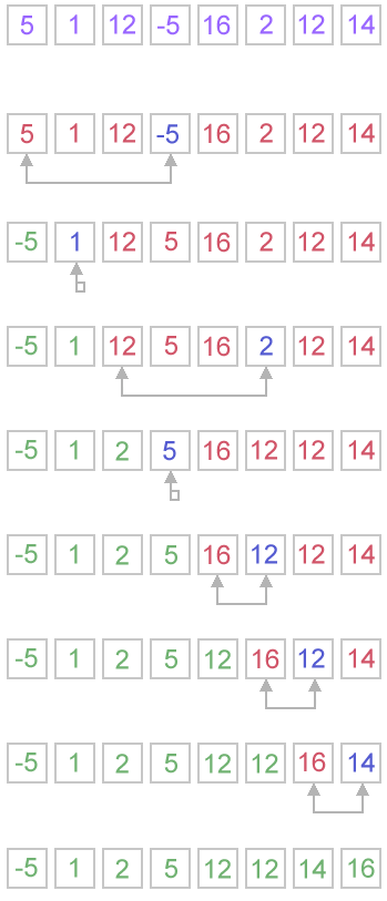
The idea of algorithm is quite simple. Array is imaginary divided into two parts - sorted one and unsorted one. At the beginning, sorted part is empty, while unsorted one contains whole array. At every step, algorithm finds minimal element in the unsorted part and adds it to the end of the sorted one. When unsorted part becomes empty, algorithmstops.

When algorithm sorts an array, it swaps first element of unsorted part with minimal element and then it is included to the sorted part. This implementation of selection sort in not stable. In case of linked list is sorted, and, instead of swaps, minimal element is linked to the unsorted part, selection sort is stable.

Let us see an example of sorting an array to make the idea of selection sort clearer.

Example. Sort {5, 1, 12, -5, 16, 2, 12, 14} using selection sort.

Complexity analysis

Selection sort stops, when unsorted part becomes empty. As we know, on every step number of unsorted elements decreased by one. Therefore, selection sort makes n steps (n is number of elements in array) of outer loop, before stop. Every step of outer loop requires finding minimum in unsorted part. Summing up, n + (n - 1) + (n - 2) + ... + 1, results in O(n²) number of comparisons. Number of swaps may vary from zero (in case of sorted array) to n - 1 (in case array was sorted in reversed order), which results in O(n) number of swaps. Overall algorithm complexity is O(n²).

Fact, that selection sort requires n - 1 number of swaps at most, makes it very efficient in situations, when write operation is significantly more expensive, than read operation.

Code snippets

Java

public void selectionSort(int[] arr) {

int i, j, minIndex, tmp;

int n = arr.length;

for (i = 0; i < n - 1; i++) {

minIndex = i;

for (j = i + 1; j < n; j++)

if (arr[j] < arr[minIndex])

minIndex = j;

if (minIndex != i) {

tmp = arr[i];

arr[i] = arr[minIndex];

arr[minIndex] = tmp;

}

Python

for i in range(len(L)-1):

minIndex = i

minValue = L[i]

j = i + 1

while j< len(L):

if minValue > L[j]:

minIndex = j

minValue = L[j]

j += 1

if minIndex != i:

temp = L[i]

L[i] = L[minIndex]

L[minIndex] = temp

ytl 2011-05-06 16:16 发表评论